The Pennsylvania State University, Spring 2021 Stat 415-001, Hyebin Song
Interval Estimation
Interval EstimationIntroduction to Interval EstimationLearning objectivesInterval estimators and interval estimatesSteps to construct an interval estimator for using a pivotal quantityConfidence intervals for one mean Learning objectivesConfidence intervals for one meanSummaryConfidence Intervals for the difference of two meansLearning objectivesTwo independent random samples vs a paired random sampleConfidence intervals for the difference of two meansSummaryConfidence intervals for proportionsLearning objectivesConfidence interval for one proportionConfidence interval for the difference of proportions
Introduction to Interval Estimation
Learning objectives
- Understand the concepts of interval estimators, confidence coefficients, and and interval estimates
- Understand how to construct and interpret confidence intervals.
Interval estimators and interval estimates
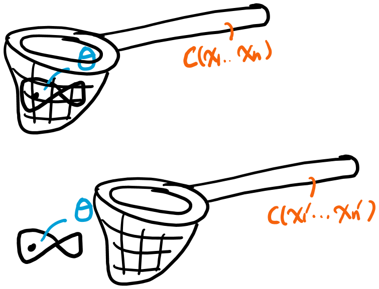
Definitions
Interval estimator for : a random interval such that , which is designed to infer a specific parameter .
- We construct and so that an interval estimator contains at least % times. In other words,
This is called the confidence coefficient .
Interval estimate for : an observed interval .
- If the corresponding interval estimator has the confidence coefficient of , the interval estimate of is also called as a % confidence interval for .
Remark
- The probability that a 95% confidence interval (a fixed interval) contains the parameter is (parameter is in the interval) or (parameter is not in the interval). If we construct many 95% confidence intervals based on many random samples, then we can expect that 95% of the realized intervals would contain the parameter.
- Since a confidence interval either covers or does not, we cannot say that is in with 95% chance.
Steps to construct an interval estimator for using a pivotal quantity
Recall that the goal is to find and such that
given a confidence coefficient .
Basic idea: use the distribution of a "good" estimator of to decide a "margin" around the point estimate.
The probability that is within the distance of is the same as the probability that is within distance of .
Choose such that . Then,
Example We have a random sample such that .
is a good estimator of . The distribution of = .
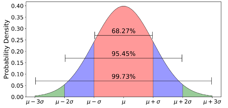
The probability that is within of %.
Equivalently, the probability that is within of %.
An interval estimator for :
- Confidence coefficient: .
Let be an realization of . The interval estimate for (=95.45% confidence interval) is .
Here are general steps:
Pick a good estimator of .
- Often, the use of "good" estimators results in good confidence intervals
Find or approximate the distribution of an estimator for .
In particular, we use one of the following three methods:
- use the exact distribution of an estimator
- use an asymptotic distribution of
- use a numerical method to approximate the distribution of
Often, we work with the distribution of a function of the estimator and the parameter , , whose distribution is known.
- Such is called as a pivotal quantity ( should not depend on any other unknown parameters than ).
Choose such that based on the distribution of or .
An interval estimator with confidence coefficient is .
Confidence intervals for one mean
Learning objectives
Know how to compute a confidence interval for when we have
- a random sample from with known
- a random sample from with unknown
- a random sample from an unknown distribution but when we have a large sample size
Confidence intervals for one mean
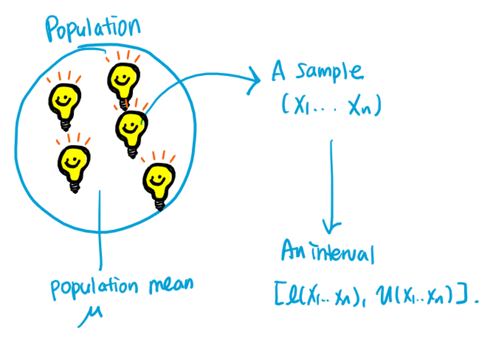
1. Confidence interval for when with known.
Example: Let equal the length of life of a 60-watt light bulb marketed by a certain manufacturer. Assume that the distribution of is . A random sample of bulbs is tested until they burn out, yielding a sample mean of hours. Find a 90% and 95% confidence interval for .
First, we need to find an interval estimator with the confidence coefficient . That is, find and such that
Then, the realized interval is a confidence interval for . How can we find such and ?
We follow the four steps to construct an interval estimator:
The statistic is a good estimator for .
Since , by the additive property of the normal distribution, .
A pivotal quantity: (recall that is known).
To choose such that , find the number such that
The number is the 1- quantile of the standard normal distribution; i.e., the number such that .
You can find the number in Table V in Appendix B of HTZ.
You can use a computer software, such as R, to look up the quantile of the standard normal distribution to find . For example, if you want to find in R, you can run
qnorm(0.975,mean = 0,sd = 1) #0.975(=1-0.025) quantile of the standard normal distto find .
We have .
- Then, we have .
- An interval estimator for with the confidence coefficient of = .
- A confidence interval for = .
Therefore, 90% and 95% confidence intervals for the average length of life of a 60-watt light bulb are
- 90% confidence interval ():
- 95% confidence interval ():
Remark In practice, one can never "know" whether the data are from a normal distribution or not. Often, people perform some sorts of normality tests to determine if an observed data set can be well-modeled by a normal distribution. One quick but powerful test is to plot a histogram of the observed data and see whether the shape of histogram resembles a bell-curve.
2. Confidence interval for when with unknown.
Example: Let equal the length of life of a 60-watt light bulb marketed by a certain manufacturer. Assume that the distribution of is normal. A random sample of bulbs is tested until they burn out, yielding a sample mean of hours and sample standard deviation of . Construct a 90% and 95% confidence interval for .
We construct a confidence interval for when is unknown. Following 4 steps,
We use as an estimator of .
Since each i.i.d., we have, .
We have . This is a function of , and unknown (not a function of and anymore). We replace the unknown population variance with the sample .
Thus a pivotal quantity .
Lemma: , "t-distribution" with a degrees of freedom of .
proof.
(Theorem 5.5-3 in HTZ) If , , and are independent, then .
(Theorem 5.5-2 in HTZ) For i.i.d., we have,
- and are independent.
In other words, .
Combining two theorems,
Find the number such that
The number is the 1- quantile of a t distribution with degrees of freedom; i.e., the number such that .
You can find the number it Table VI in Appendix B of HTZ for some commonly used values.
You can use a computer software, such as R, to look up the value of . For example, the script
xxxxxxxxxxqt(0.975,df = 10) #0.975(=1-0.025) quantile of the t dist with df = 10returns .
Therefore, . In other words,
- An interval estimator for with the confidence coefficient of : .
- A confidence interval for = .
Therefore, 90% and 95% confidence intervals for the average length of life of a 60-watt light bulb are
90% confidence interval ():
- In R,
qt(0.95,df=26)returns 1.70
- In R,
95% confidence interval ():
- In R,
qt(0.975,df=26)returns 2.01
- In R,
Remark: we see that and , and thus the length of confidence intervals when is unknown is longer than the confidence intervals when is known. This is because distribution has a thicker probability tail than the standard normal distribution.
In fact, any distribution with a finite degrees of freedom has a thicker tail than the standard normal distribution, and as the degrees of freedom increases, the t distribution becomes more similar to a normal distribution. Usually, when the degrees of freedom is over 30, distribution is quite similar to the standard normal distribution.
3. Confidence interval for with an unknown underlying distribution and large
Example: Let equal the length of life of a 60-watt light bulb marketed by a certain manufacturer. A random sample of bulbs is tested until they burn out, yielding a sample mean of hours. From previous study, it is known that . Construct an approximate 90% and 95% confidence interval for .
Since we do not know the distribution of , it would be hopeless to find the exact distribution of . Luckily, we have a large sample size (), and thus we can use the CLT to obtain
Note: even though we know the distribution of , it is often hard to obtain the exact distribution of . In such cases, we can use this normal approximation instead.
From (1), we have,
Then,
Thus we have,
- an (asymptotically correct) interval estimator for with the confidence coefficient of = .
- an approximate confidence interval for = .
Remark: Here, an "asymptotically correct" interval estimator means the random interval covers the parameter % when is large. In other words, the inequality, ,
is "correct" when is large ("asymptotic").
Therefore, approximate 90% and 95% confidence intervals for the average length of life of a 60-watt light bulb are
- 90% confidence interval ():
- 95% confidence interval ():
Suppose the previous knowledge on the population variance was unavailable. In such case, we replace the population variance with the sample variance and use the following approximation:
this is due to the fact that when is large (more precisely, is a consistent estimator for .)
Then, following similar steps as before, we have,
- an (asymptotically correct) interval estimator for with the confidence coefficient of = .
- an approximate confidence interval for = .
In particular, we can use the same approximate 90% and 95% confidence intervals for the average length of life of a 60-watt light bulb even though the population variance is replaced with the sample variance.
Summary
When we have the observed sample from a random sample ,
| Settings | confidence interval |
|---|---|
| , known | |
| , unknown | |
| Any distribution with , known, large | (approximate) |
| Any distribution with , unknown, large | (approximate) |
Remark: the normal approximation of the distribution of is in general quite good, especially when the distribution of is symmetric, unimodal, and of the continuous type. When the distribution of is highly skewed, a larger sample size is needed for the approximation to be reasonably accurate.
In particular, when the sample size is small and is not normally distributed (especially when heavily skewed), it is preferred to use a numerical method to directly approximate the distribution of .
Confidence Intervals for the difference of two means
Learning objectives
Understand the difference of independent and paired random samples
Know how to compute a confidence interval for the difference of two population means when we have
- two independent random samples , from and with known and .
- two independent random samples , from and with unknown variances (two cases: 1. common variance , 2. different variances )
- two independent random samples , from unknown distributions but when we have large sample sizes and .
- two paired random samples
Two independent random samples vs a paired random sample
Suppose a researcher wants to study whether lack of sleep impacts cognitive performance.
Protocol 1: The researcher recruited 20 participants and divided them into 2 groups. The participants in the first group are allowed to have a normal sleep, but people in the second group are kept awake for 24 hours. Results of cognitive tests are recorded for each patient. Let be the test score result for the th participant from the first group, and be the test score result for the th participant from the second group.
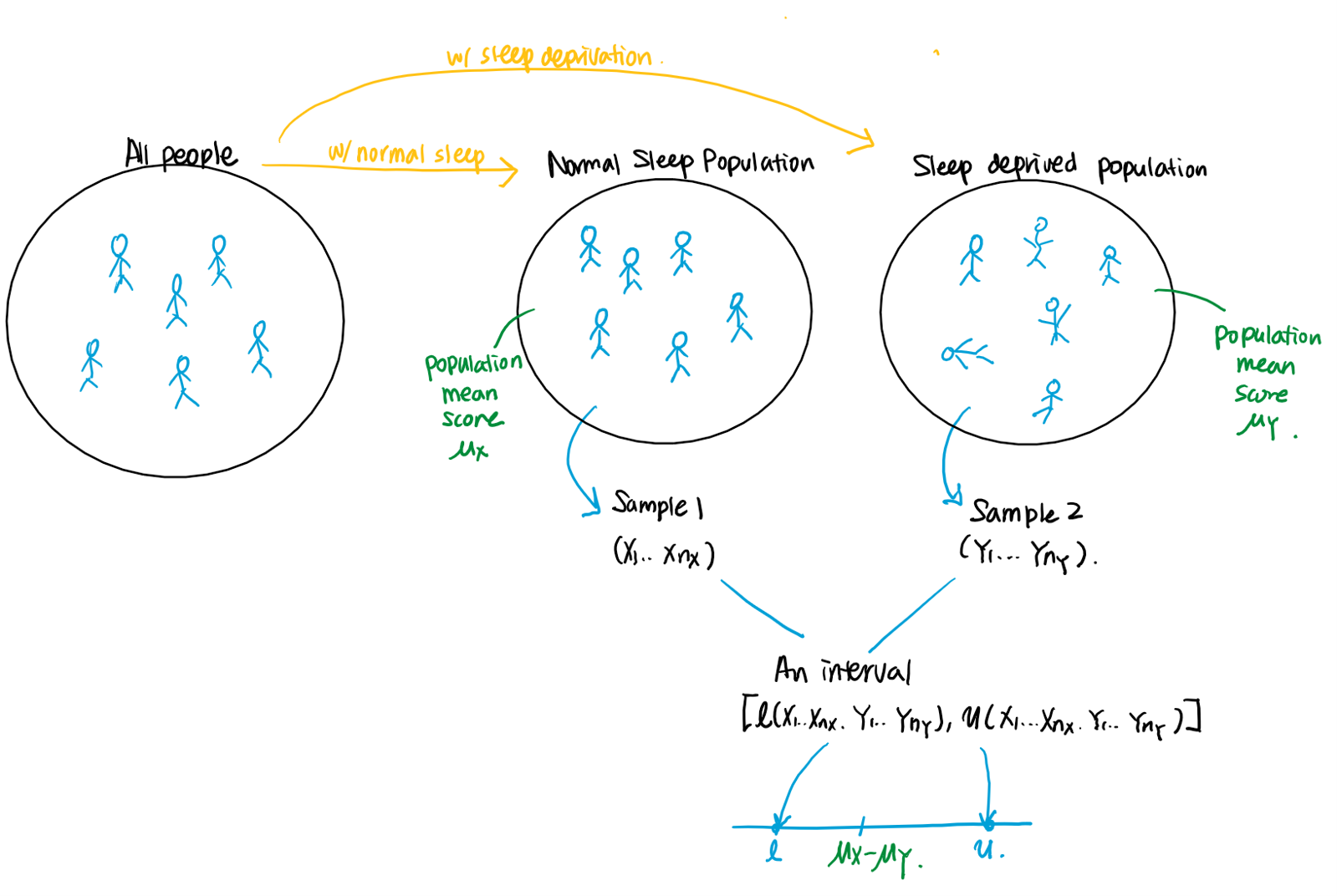
Protocol 2: The researcher recruited 10 participants. Each participant is asked to take the tests twice: one after a normal sleep and the other after being kept awake for 24 hours. Let be the first test score result for the th participant, and be the second test score result for the th participant .
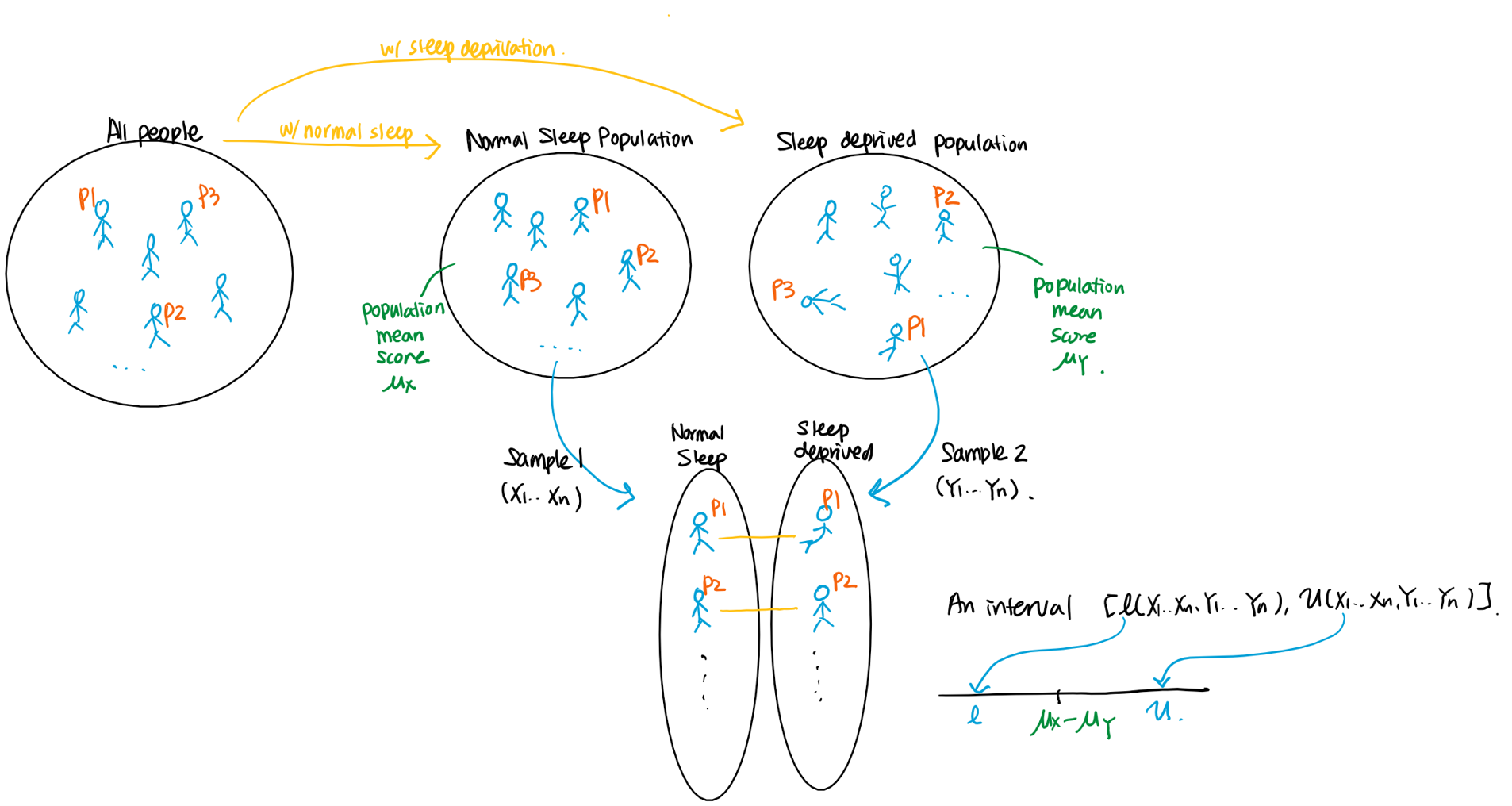
In the first protocol, there is no association between th subject from the first and second group, and therefore and are independent. On the other hand, in the second protocol, and are dependent, since the test results are from the same th person. In fact, we have a paired random sample, since each and should be paired. Therefore,
- Following the first protocol, we would have two independent random samples and .
- Following the second protocol, we would have a paired random sample .
Confidence intervals for the difference of two means
1. Confidence interval for the difference of the population mean from two independence normal random samples with known variances
Example The researcher followed the first protocol and obtained the following data:
| Group | Scores | |
|---|---|---|
| Group 1 (normal sleep) | 8.4, 9.2, 8.2, 10.6, 9.3, 8.2, 9.5, 9.7, 9.6, 8.7 | |
| Group 2 (awake for 24 hours) | 8.5, 7.4, 6.4, 4.8, 8.1, 7.0, 7.0, 7.9, 7.8, 7.6 | |
Let and equal the test score of a participant in the first and second group. Based on previous studies, the researcher decided that it is reasonable to assume that the distribution of test scores is normal with the variance of . The researcher wants to form a 95% confidence interval for the difference of test scores between two groups.
Let and be unknown population means of group 1 and 2. We need to find an interval estimator with the confidence coefficient . That is, find and such that
We follow the four steps to find an interval estimator:
We use an estimator for .
The distribution of is (using independence of and )
The pivotal quantity:
Find such that
Therefore, .
Rearranging the terms in the event,
Therefore,
An interval estimator for with the confidence coefficient of = .
A confidence interval for :
A 95% confidence interval for the difference of test scores between group 1 and group 2 is
In R,
xxxxxxxxxxgroup1 = c(8.4, 9.2, 8.2, 10.6, 9.3, 8.2, 9.5, 9.7, 9.6, 8.7)group2 = c(8.5, 7.4, 6.4, 4.8, 8.1, 7, 7, 7.9, 7.8, 7.6)xbar = mean(group1) # compute the sample mean of group 1 dataybar = mean(group2) # compute the sample mean of group 2 datamargin = qnorm(1-0.025)*sqrt(1/10 + 1/10)CI_for_diff = c(xbar-ybar - margin, xbar-ybar + margin) # 95% CICI_for_diff[1] 1.013477 2.766523
2. Confidence interval for the difference of the population mean from two independence normal random samples with unknown variances
Example: Consider the previous sleep study example. However, now the researcher is unsure about whether it is valid to assume that the population variance of each group is . The prior studies indicate that the variances of the scores from each group are likely to be the same. The researcher wants to form a 95% confidence interval for the difference of test scores between two groups.
2-1. Common variance
In Step 3, we used
as a pivotal quantity. However, in this setting where is unknown, it is not the function of data and the parameter of interest anymore. We replace with a pooled estimator of the common variance
Lemma:
proof.
Let , and such that
By theorem 5.5-3 in HTZ,
Following similar steps,
An interval estimator for with the confidence coefficient of = .
A confidence interval for :
Therefore, a 95% confidence interval for the difference of test scores between group 1 and group 2 is
In R,
xxxxxxxxxxgroup1 = c(8.4, 9.2, 8.2, 10.6, 9.3, 8.2, 9.5, 9.7, 9.6, 8.7)group2 = c(8.5, 7.4, 6.4, 4.8, 8.1, 7, 7, 7.9, 7.8, 7.6)xbar = mean(group1) # compute the sample mean of group 1 dataybar = mean(group2) # compute the sample mean of group 2 datasp2 = (sum((group1-xbar)^2) + sum((group2-ybar)^2))/18 # pooled sample variancemargin = qt(1-0.025,df = 18)*sqrt(sp2/10 + sp2/10)CI_for_diff = c(xbar-ybar - margin, xbar-ybar + margin) # 95% CICI_for_diff[1] 1.022947 2.757053
2-2. Uncommon variances
When two samples do not share the common variance, we can no longer use the pooled estimator. We replace and with and in (2) and use
as a pivotal quantity.
Although does not have the t distribution anymore, it approximately follows a t distribution with degrees of freedom (Welch, 1949) where
Using Welch's approximation,
An approximate interval estimator for with the confidence coefficient of = .
A confidence interval for :
3. Confidence interval for the difference of the population mean from two independence random samples with unknown distributions
Example The researcher decided to follow the first protocol to study the effect of sleep deprivation. The researcher first looked at some of previous literature and found out that some of the scores from previous studies had a skewed distribution. Worried about possible non-normality of test scores, the researcher recruited 100 participants (50 participants per group) and carried out experiments. Plotting histograms of test scores from each group, the researcher concluded that test scores are not likely to be from normal distributions. The researcher wants to form a 95% confidence interval for the difference of test scores between two groups.
| Group | Sample mean | Sample variance |
|---|---|---|
| Group 1 | 9.114 | 0.811 |
| Group 2 | 6.963 | 0.918 |
We have two independent random samples , from unknown distributions (but not normal) and sufficiently large and .
From an application of a version of CLT, we have
and
since and when and are sufficiently large.
Using (2) and (3),
An approximate confidence interval for with known variances:
An approximate confidence interval for with unknown variances:
Therefore, an approximate 95% confidence interval for the difference of test scores between group 1 and group 2 is
4. Confidence interval for the difference of the population mean from a paired random samples
Example A researcher wants to study whether lack of sleep impacts cognitive performance. The researcher recruited 10 participants. Each participant is asked to take the tests twice: one after a normal sleep and the other after being kept awake for 24 hours.
| 1 | 2 | 3 | 4 | 5 | 6 | 7 | 8 | 9 | 10 | |
|---|---|---|---|---|---|---|---|---|---|---|
| First test (normal sleep) | 8.1 | 9.5 | 7.2 | 11.6 | 9.9 | 7.3 | 10 | 10.7 | 10.4 | 8.5 |
| Second test (awake for 24 hours) | 7.0 | 8.6 | 6.3 | 10.7 | 8.8 | 6.3 | 8.9 | 9.1 | 9.0 | 7.5 |
Suppose it is reasonable to assume that the difference of test scores is normally distributed.
Since and are paired, we cannot use previous intervals because and are dependent (Observe that a participant who scored high in the first test tended to score high in the second test).
The key idea is to consider another random variable , which is the difference between and . Note, . Therefore the problem becomes to find a confidence interval for where we have a random sample of , and we can use the results from the previous lecture. Since it is assumed that and is unknown, we can use a confidence interval based on the t distribution.
Therefore, the 95% confidence interval for the difference is
where and are sample mean and variance of differences of test scores.
In R,
xxxxxxxxxxfirst = c(8.1, 9.5, 7.2, 11.6, 9.9, 7.3, 10, 10.7, 10.4, 8.5)second = c(7, 8.6, 6.3, 10.7, 8.8, 6.3, 8.9, 9.1, 9, 7.5)diff = first - second # compute the difference of scoresdmean = mean(diff)# sample meandvar = var(diff) # sample variancemargin = qt(1-0.025,df = 9)*sqrt(dvar/10)CI_for_diff = c(dmean - margin, dmean + margin) # 95% CICI_for_diff[1] 0.9347954 1.2652046
Summary
When we have the observed sample , from two random samples ,
| Settings | confidence interval |
|---|---|
| , , independent, known | |
| , , independent unknown | |
| , , independent unknown | where s the df from Welch's approximation |
| Two independent random samples, large and | (approximate) , or |
| Paired samples (dependent, ), when , unknown | |
| Paired samples (dependent, ), large | (approximate) |
where
- is a pooled sample variance estimate,
- is a sample variance estimate from ,
- is a sample variance estimate from ,
- is a sample variance estimate from where .
Confidence intervals for proportions
Learning objectives
- Know how to compute a confidence interval for the population proportion
- Know how to compute a confidence interval for the difference of population proportions
Confidence interval for one proportion
Suppose we have a random sample . The goal is to construct an approximate confidence interval for when is large. Note that (for any ). By CLT, we have,
Note is (asymptotically) pivotal, since it depends only on and (and does not depend on any unknown parameter).
In step 3, we choose such that
Unlike previous cases, both numerator and denominator depend on .
1. Wald Confidence Intervals:
Since when is large ( is a consistent estimator of ),
Therefore, we have,
In other words,
- an (asymptotically correct) interval estimator for with the confidence coefficient of = .
- an approximate confidence interval for = .
2. Wilson Confidence Intervals:
Rewriting, we get
, and
In other words,
By the quadratic formula, we can show that
an (asymptotically correct) interval estimator for with the confidence coefficient of :
an approximate confidence interval for :
Remarks:
Both the Wilson and Wald confidence intervals are valid asymptotically (large ): they both have asymptotic confidence coefficient
- When is large, , and are small, thus Wilson and Wald confidence intervals are approximately equal.
In some scenarios, especially for small and/or near 0 or 1, the Wald confidence interval performs badly
The endpoints of the Wilson confidence interval are guaranteed to be within , whereas the Wald CI may have upper or lower bounds outside of (which doesn't make sense for proportions)
The Wilson confidence interval often has better coverage probability than the Wald interval
For these reasons, the Wilson confidence interval is sometimes recommended over the Wald confidence interval
Confidence interval for the difference of proportions
Suppose we now have two independent random samples , . The goal is to construct an approximate confidence interval for the difference of when are large.
From an application of a version of CLT, we have
and
Therefore,
an (asymptotically correct) interval estimator for with the confidence coefficient of = .
an approximate confidence interval for :
.
Example A random sample of men produced a total of who favored a controversial local issue. An independent random sample of women produced a total of who favored the issue. Assume that is the true underlying proportion of men who favor the issue and that is the true underlying proportion of women who favor of the issue. Find a 95% confidence interval for .
Let be the preference of the ith men, and be the preference of the ith women.
We have and . The observed sample means are .
An approximate 95% confidence interval for is